How one can Disguise Zero Values in Excel Charts

Editor’s observe: Within the video, Brandon Vigliarolo walks you thru a few methods to suppress 0 values in Excel charts. For this demo, he makes use of Microsoft Workplace 365. The steps are just like what Susan Harkins describes within the following tutorial.

A drop to zero in a chart will be abrupt, however generally, that’s what you need. However, there can be occasions once you received’t need to draw consideration to a zero. If you don’t need to show zero values, you’ve gotten a couple of decisions for hiding or in any other case managing these zeros.

On this tutorial, I’ll evaluation a couple of strategies for dealing with zero values that provide fast however restricted outcomes with minimal effort. Relying on how a lot charting you do, you may discover multiple of those strategies useful.

Following alongside

For this demonstration, I’m utilizing Microsoft 365 Desktop on a Home windows 11 64-bit system, however you can too use earlier variations of Excel. Excel for the net helps most of those strategies.

SEE: Google Workspace vs. Microsoft 365: A side-by-side evaluation w/guidelines (TechRepublic Premium)

You’ll be able to comply with alongside extra carefully by downloading our demonstration file. In the event you work by means of the directions utilizing our demonstration workbook file, undo every answer earlier than you begin the subsequent. You are able to do this by merely closing the file and reopening it with out saving it.

Exploring the pattern dataset

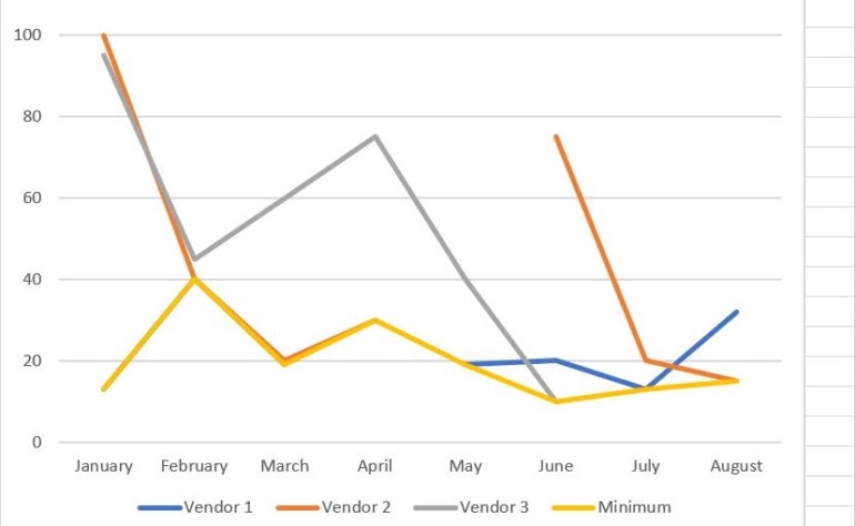
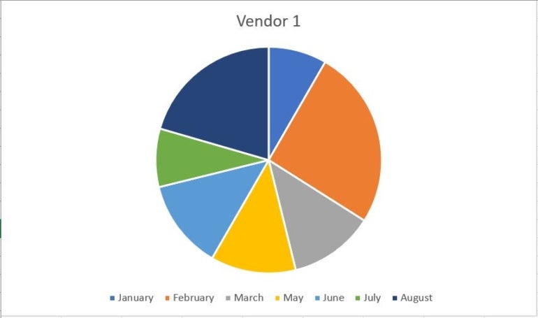
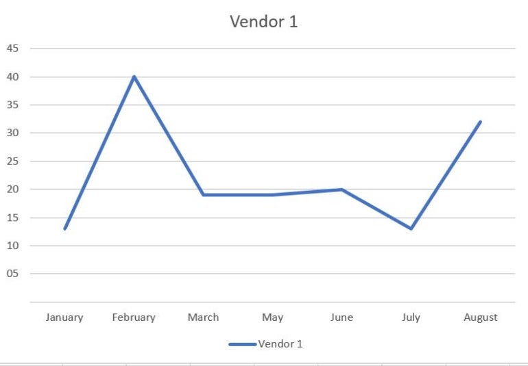
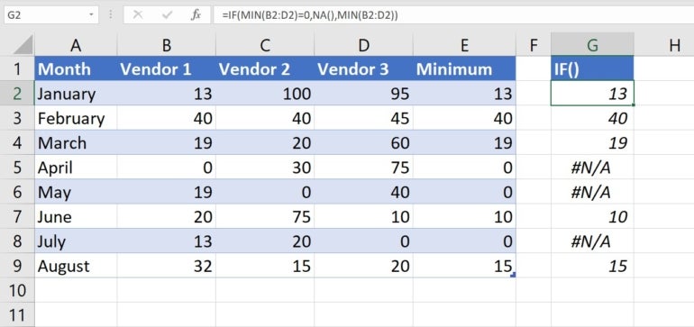
The instance beneath exhibits the info and preliminary charts that we’ll replace all through this text. The pie and single-line charts mirror the info in column B for Vendor 1. The opposite two charts have three information sequence: Vendor 1, Vendor 2, and Vendor 3. The Minimal column returns the minimal worth for every month, so April, Ma, and July return zero for the minimal worth. This setup simplifies all of the examples we’ll be reviewing on this information.

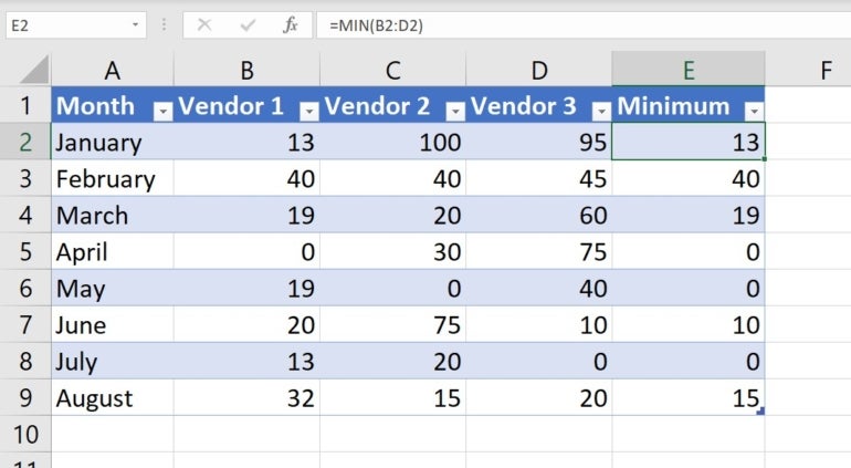
Proper now, the charts show zero values by default in every chart kind.

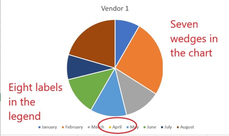
Pie chart

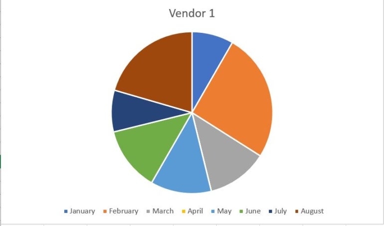
By default, the pie chart, proven beneath, charts the zero, however you’ll be able to’t see it. In the event you activate information labels, you will notice the zero listed. There are seven slices however eight objects within the legend.

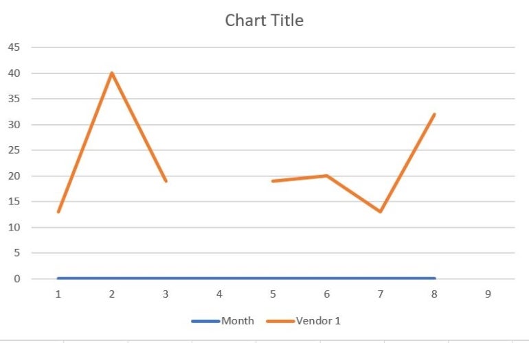
Line chart

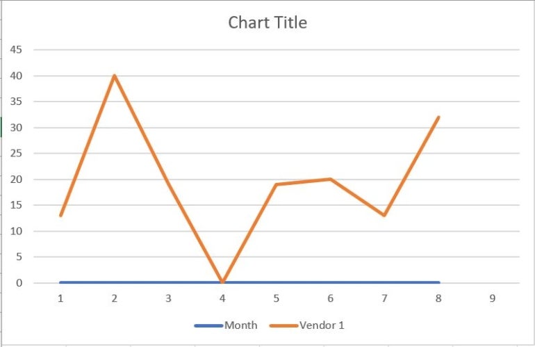
The beneath instance exhibits the road chart’s default conduct, which drops the one to zero on the X-axis.

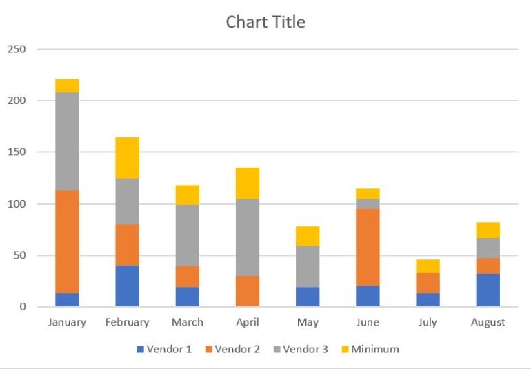
Stacked bar chart

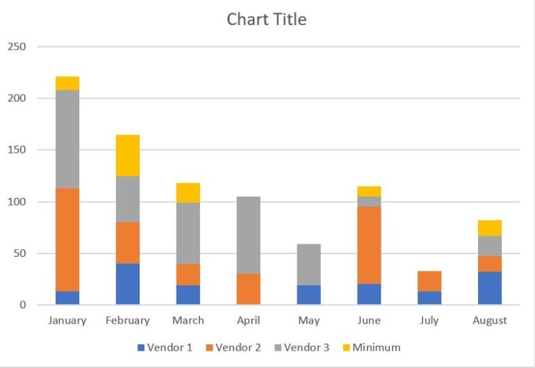
Excel plots 4 stacks for the months with no zero worth within the stacked bar chart proven beneath. The months with a zero show solely two values as a result of the Minimal column additionally returns zero for these months, so the chart is definitely plotting two zeros for every month. Readers is perhaps a bit confused by what they’re seeing.

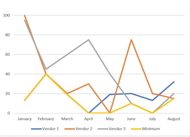
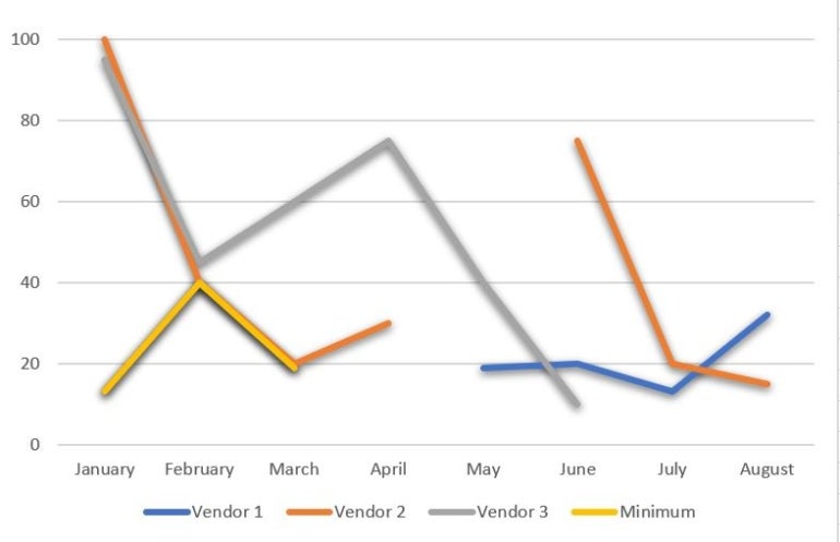
A number of-line chart

This multiple-line chart beneath is messy; enlarging it doesn’t enhance its readability. Though you’ll be able to’t see all the strains, they’re there. The values are so shut that some strains obscure the others, which is deceptive.

Your outcomes could fluctuate relying on Excel’s default settings and theme colours. Now that you realize the instance information, let’s evaluation a couple of strategies for suppressing the zero values in our instance charts. Some will work with restricted outcomes, and others received’t work in any respect.

Eradicating and formatting zero

There’s multiple method to suppress zero values in a chart, however none work the identical persistently for all charts.

Guide removals of zero

To start with, you may strive eradicating zero values altogether if it’s a literal zero and never the results of a method. By eradicating, I imply merely deleting all zero values from the dataset. Sadly, this easiest strategy doesn’t all the time work as anticipated.

Pie chart

The pie chart doesn’t chart the clean cell, however the legend nonetheless shows the class label, as proven beneath. Eradicating the zero values from the dataset modified nothing.

Stacked bar chart

The stacked bar responds apparently. It doesn’t chart the zero values, however as a result of the zeros are gone, the MIN() features within the Minimal column are actually all non-zero values and chart accordingly.

Line and multiple-line charts

Neither line chart handles the lacking zeros nicely, however the multiple-line chart is hopeless. The road chart has a niche between the 2 months, which undoubtedly appears odd.

The multiple-line chart is misleading. The Vendor 1 sequence seems improper, however you will notice the markers if you happen to click on it. It’s there however obscured by different strains; even doubling its measurement does nothing to enhance its readability.

In the event you eliminated zero values within the sheet throughout this section, re-enter them earlier than persevering with to our subsequent instance. Or, shut the demonstration file with out saving your adjustments and reopen it.

Unchecking worksheet show choices

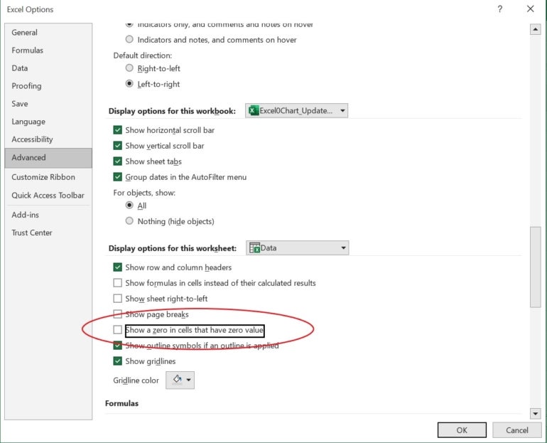
It’s also possible to conceal zeros by unchecking the worksheet show possibility referred to as Present A Zero In Cells That Have Zero Worth. Right here’s how:

1. Click on the File tab and select Choices. You may need to click on Extra first.
2. Select Superior within the left pane.
3. Within the Show Choices For This Worksheet part, select the best sheet from the drop-down menu. (It is a sheet-level property.)
4. Uncheck the Present A Zero In Cells That Have Zero Worth possibility.
5. Click on OK.

The zero values nonetheless exist — you’ll be able to see them within the Formulation bar. Nonetheless, Excel received’t show them; thus, this methodology has no influence. The charts deal with the zero values as in the event that they’re nonetheless there as a result of they’re. Excel for the net doesn’t enable entry to this setting.

We’ve discovered that unchecking this setting affords no benefit. I embody this step in our tutorial to forestall you from losing your time on this system your self.

Setting a customized format

Earlier than you do this subsequent formatting possibility, reset the Superior possibility that you simply disabled in our earlier step, or shut the file with out saving and reopen it. Take into accout this subsequent formatting strategy has diversified outcomes. Right here’s the way it works:

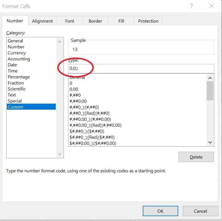
1. Choose the info vary B2:D9.
2. Click on the Quantity group’s dialog launcher (Residence tab).
3. Within the ensuing dialog field, select Customized from the Class checklist.
4. Within the Kind management, enter 0,0;;; and click on OK.

You’ll discover that the outcomes are just like these seen earlier:

• Pie chart: The pie chart doesn’t chart the zero worth, however April continues to be within the legend.
• Stacked bar chart: The stacked bar chart shows solely two stacks for the months with a zero worth.
• Line and multiple-line charts: Each line charts embody zero values.

As a result of these strategies are really easy to use, strive deleting or formatting the zeros first. Nonetheless, it’s vital to acknowledge that these strategies won’t possible replace all charts the way you need. You may need to discover a completely different answer for every chart!

In the event you utilized this format to the demonstration file, delete it earlier than you proceed. Or shut the file with out saving it after which reopen it.

SEE: Right here’s find out how to enter main zeros in Excel

Charting a filtered dataset

In case you have a single information sequence, you’ll be able to filter out the zero values and chart the outcomes. Just like the strategies mentioned above, it’s a restricted alternative as a result of you’ll be able to solely chart one vendor at a time. Moreover, Excel for the net doesn’t assist this system.

SEE: 10 tricks to make your Excel spreadsheets look skilled and practical 

Let’s exhibit. Begin by including a filter to the Vendor 1 column with these steps:

1. Click on inside the info vary.
2. On the Knowledge tab, click on Filter within the Kind & Filter group. In the event you’re working with a Desk object, you’ll be able to skip this step as a result of the filters are already there.
3. Click on Vendor 1’s drop-down and uncheck zero.

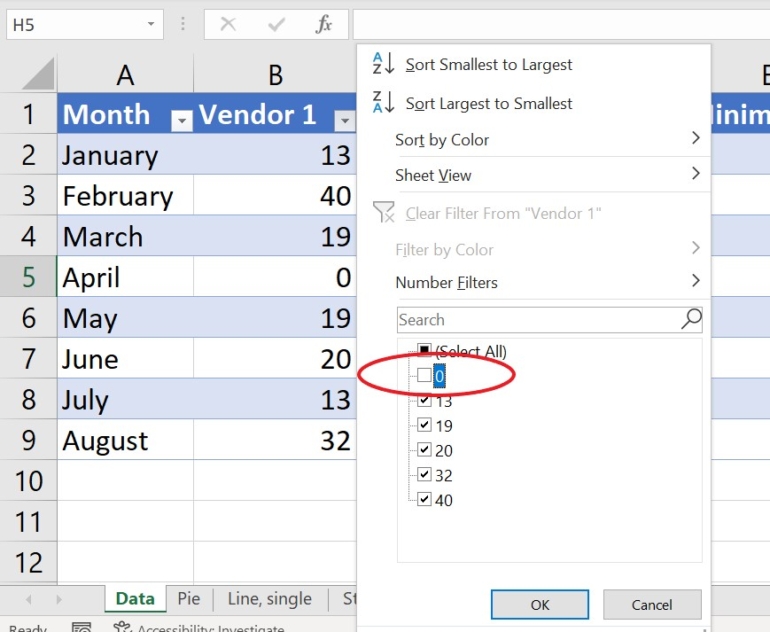
4. Click on OK to filter the column, which is able to filter your entire row. Don’t fear about that, however make sure you take away the filter once you’re completed.

The beneath instance exhibits the brand new pie chart.

Under, you’ll be able to see the brand new line chart.

Each charts are based mostly on the filtered information in column B. Neither shows the zero worth or the class label on the X-axis. Nonetheless, the road chart has a severe flaw: The road is stable, and April has the identical worth as March. Distributing this chart as-is can be a severe mistake as a result of the info for April is inaccurate.

Sadly, once you take away the filter, the charts replace and show the zero values. However, in case your chart is a one-time job, filtering affords a fast repair for a pie chart.

In the event you tried this with the demo file, undo the change, shut it with out saving it, and reopen it.

Change zeros with NA()

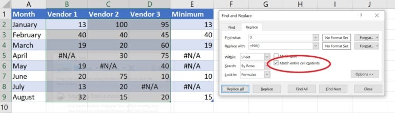
Essentially the most everlasting repair for hiding zeros is to exchange literal zero values with the NA() perform utilizing Excel’s Discover and Change characteristic. In the event you replace the info recurrently, you may even enter NA() for zeros from the get-go, eliminating the issue altogether. To take action manually, enter =NA(). Nonetheless, that’s not all the time sensible, so let’s use Excel’s Change characteristic to exchange the zero values within the instance dataset with the NA() perform:

1. Choose the dataset. On this case, it’s B2:D9.
2. Click on Discover & Choose within the Modifying group on the Residence tab after which select Change from the dropdown, or press Ctrl + H.
3. Enter 0 within the Discover What management.
4. Enter =NA() within the Change management.
5. If vital, click on Choices to show extra settings.
6. Examine the Match Total Cell Contents possibility.

7. Click on Change All, and Excel will exchange the zero values.
8. Click on OK to dismiss the affirmation message.
9. Click on Shut.

The determine above exhibits the settings and the outcomes. In the event you don’t choose the Match Total Cell Contents possibility in step six, Excel will change the values 40, 404, and so forth. The formulation in column E show the error worth as a result of they reference a cell that shows the error message.

Not one of the charts show the #N/A error values, however they nonetheless show the class label within the axis and the legend. The stacked bar chart shows solely two stacks for the months with a #N/A worth, so there’s no distinction. The one curiosity is the multiple-line chart: The zero values, which are actually #N/A error values, are clearly seen.

Suppose you’re working with the outcomes of formulation that may return zero as a substitute of an error worth. In that case, you should use an IF() perform to return the #N/A error utilizing the next syntax:

=IF(method=0,NA(),method)

The MIN() perform returns the minimal worth for every month. The IF() perform returns #N/A if the result’s zero:

=IF(MIN(B2:D2)=0,NA(),MIN(B2:D2))

The instance’s contrived, however don’t let that trouble you. The reality is, you’re unlikely to want this expression as a result of most features and expressions return the #NA error worth in the event that they attempt to consider one.

Selecting from chart settings to chart zero values

A number of charts present a niche between one worth and one other when the zero worth is lacking. In the event you’re working with one chart, you’ll be able to rapidly bypass the guesswork by utilizing a chart setting to find out find out how to chart zero values. Right here’s how:

1. Choose the chart.
2. Click on the contextual Chart Design tab.
3. Within the Knowledge group, click on Choose Knowledge.
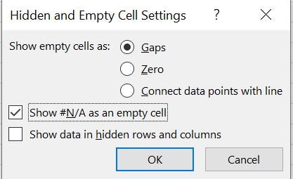
4. Within the ensuing dialog, click on the Hidden and Empty Cells button within the bottom-left nook.

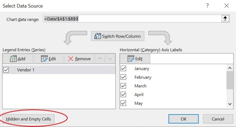
5. Select one of many choices.

6. Click on OK twice to return to the chart.

How do you exclude zero in information labels?

There’s no simple method to take away the zero in information labels. If the chart doesn’t chart it, more often than not, it received’t show the worth in a knowledge label. After working by means of all these examples, you’ll be able to see that the problem comes with no ensures. You’ll should discover a bit to search out the best settings.

If the chart doesn’t show the zero within the chart or the info label however does show the sequence within the legend, you’ll be able to take away it. Merely choose that merchandise within the legend and press Delete. In the event you by accident delete all of them, press Ctrl + Z to undo the delete and take a look at once more, ensuring to pick solely the one label you need to take away.

Last suggestions

There isn’t a simple one-size-fits-all answer for zeroless charts. In the event you show zeros for reporting functions however don’t need to see them in charts and also you chart typically, take into account sustaining two datasets: one for reporting and one for charting. That is the most effective various to toggling backwards and forwards with one dataset.

The true downside is the story the info tells. Zero is a sound worth and Excel treats it as such.

Learn subsequent: Discover a number of the finest free alternate options to Microsoft Excel.